Scientific tutorial · Computational Atomic-Resolution STEM: Concepts and Methods · Scientific Computing ·
When Can We Add Atomic Images Together?
An evidence-synchronized visual guide to when HAADF-STEM atomic responses can be added, how geometry changes non-additivity, and when higher image order is needed.
How to use this tutorial
This is one tutorial with three reading depths rather than three separate versions. Core: follow the main story, figures, findings, and limitations. Technical: add the Methods depth when you want the construction of matched subsets, simulation controls, validation, and numerical checks. Expert/reproducibility: add Technical depth, equations, provenance, and Sources for the formal decomposition and evidence boundaries. Start with the Core route and open deeper layers only when useful; no other tutorial is a prerequisite.
Learning objectives
By the end of the Core route, you should be able to explain why a HAADF-STEM atomic feature is an imaging response rather than a literal atom picture; distinguish one-body addition, pair corrections, and a residual beyond pair order; explain why transverse and beam-direction separations must be treated separately; distinguish full-image error from error normalized by a weak interaction residual; state what the tested Au2/Au3 evidence supports and does not support; and explain why the 0.75 Å applicability boundary is operational rather than a universal physical threshold.
Start with what the microscope measures
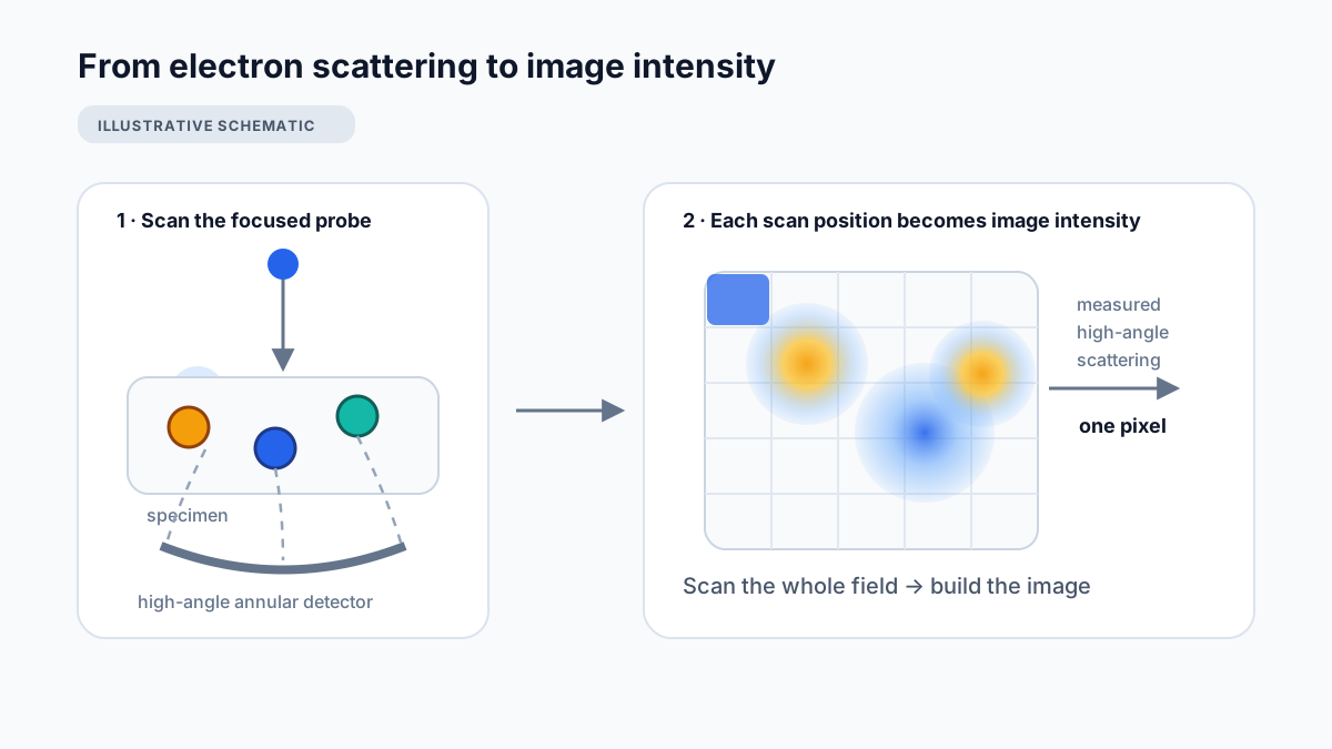
HAADF-STEM—high-angle annular dark-field scanning transmission electron microscopy—moves a focused electron probe across a specimen. At each probe position, a detector records electrons scattered into a high-angle annular range. Repeating that measurement across the scan builds a two-dimensional intensity map.
The bright features are therefore not literal photographs of spherical atoms. They are the microscope response produced by electron–specimen interaction under a particular beam, detector, geometry, sampling, and numerical configuration.
From electron scattering to image intensity
One atom gives a spatial response
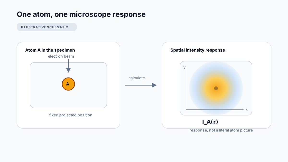
Place one gold atom in the calculation while keeping the imaging conditions fixed. The result is a spatial intensity field. We can denote the response of atom A by I_{A}(r), where r labels position in the image.
The notation is useful, but the idea is simple: one selected atom, calculated on its own under the comparison conditions, produces one matched singleton image.
One atom, one microscope response
The question
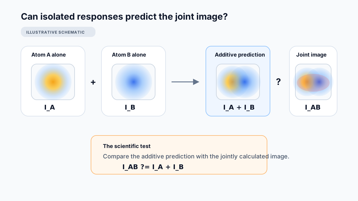
If we know the matched image produced by each atom separately, can we reconstruct the image of the atoms together simply by adding those images? If addition fails, how much extra image structure requires pair-specific or higher-order terms?
Can two isolated responses predict the joint image?
Why addition can fail
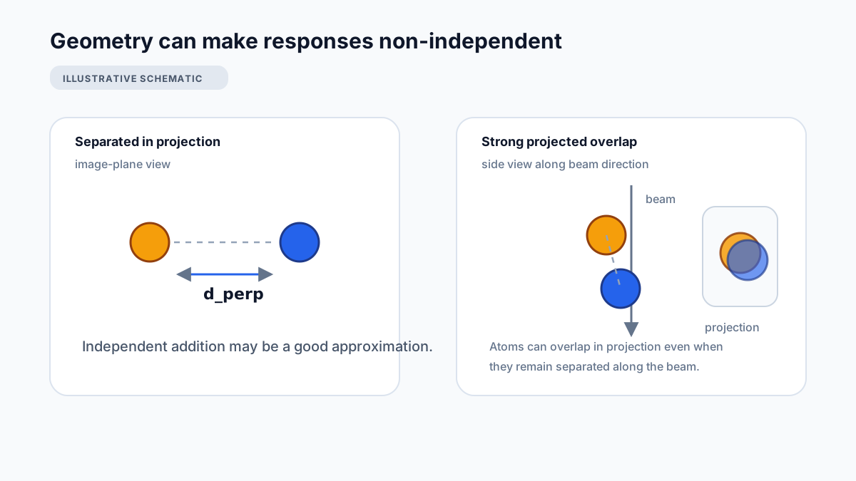
The additive construction is a hypothesis, not a law. When atoms occupy geometries that strongly couple image formation, the joint calculation can contain intensity structure absent from either isolated response. In particular, atoms separated along the beam can still lie close together in projection.
We describe their separation across the image plane by d_perp. Geometry along the beam also matters, so one distance alone does not completely describe the response.
Geometry can make responses non-independent
A worked example: pair residual
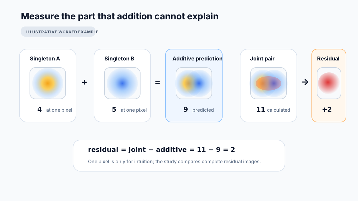
Use deliberately simple arithmetic before looking at full images. At one pixel, suppose the matched singleton calculations give intensities 4 and 5. Addition predicts 9. If the joint two-atom calculation gives 11, then the residual at that pixel is 2.
Another pixel could have a negative residual. The research does not judge the interaction from one pixel: it compares the complete images and residual fields.
Measure the part that addition cannot explain
What does matched mean?
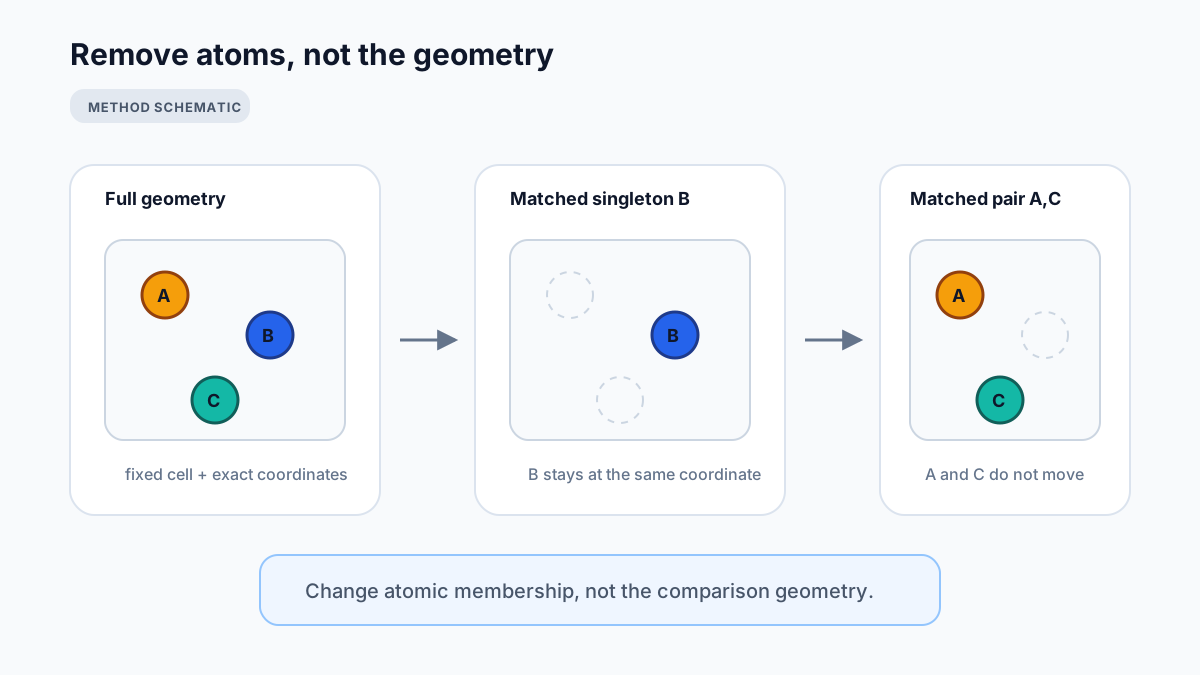
The singleton images are not generic pictures of a gold atom pasted into the scene. For a matched subset, the selected atom or atoms retain their exact positions from the complete geometry while the other atoms are removed. The fixed comparison context is preserved.
This matters because the residual should change because atoms were present together—not because we silently moved them or changed the microscope configuration.
Remove atoms, not the geometry
Methods: How matching is enforced
In the Au3 control implementation, indexed singleton and pair subsets are constructed directly from the complete fixed-cell geometry at the original coordinates. The same image grid and microscope configuration are then used for the decomposition. This makes the subtraction an operational comparison of atomic membership.
The one-body reconstruction
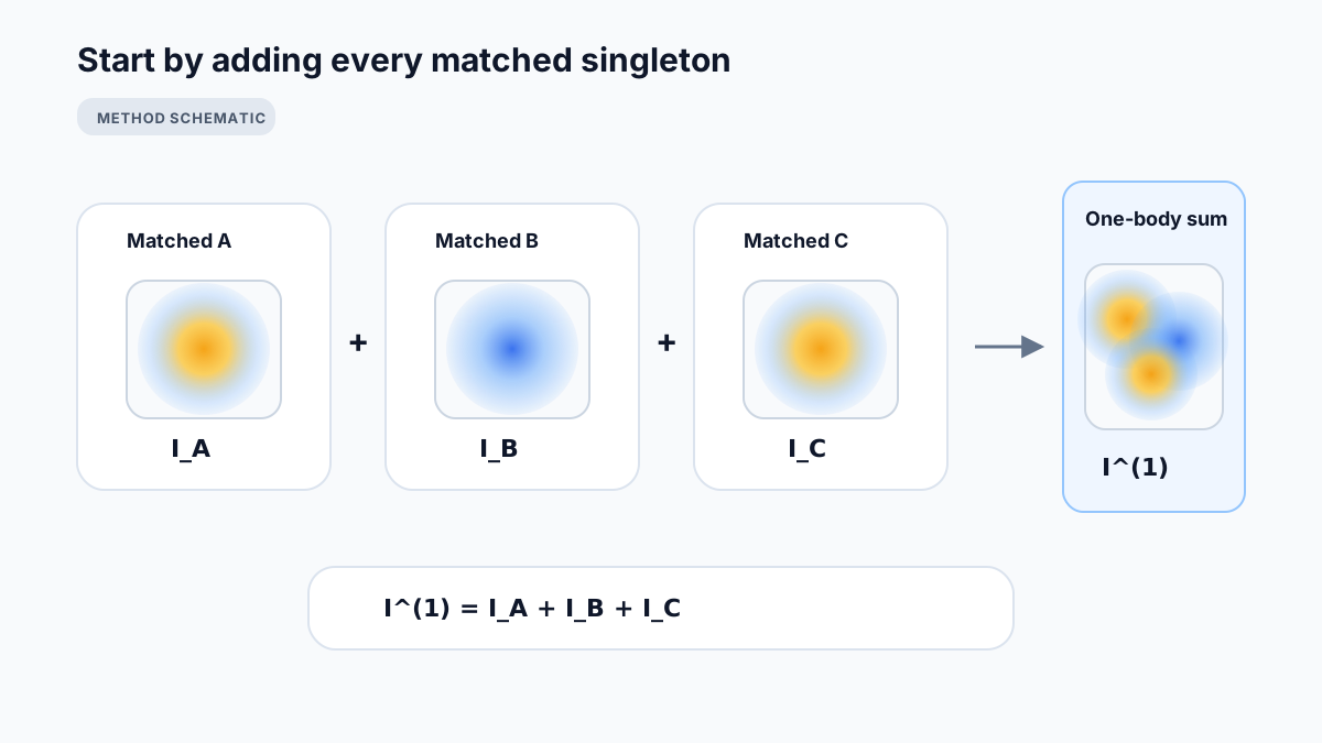
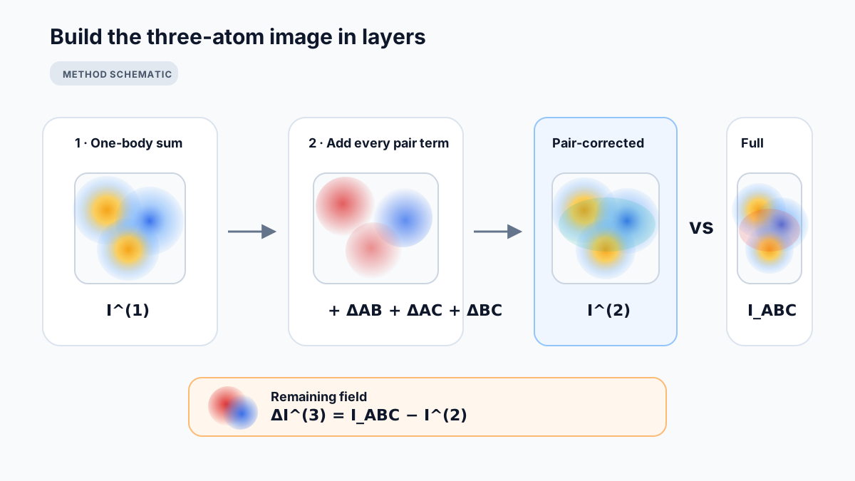
Add the matched singleton image for every atom in the structure. The superscript (1) indicates that only one-body terms have been included.
Start by adding every matched singleton
Now isolate what a pair adds
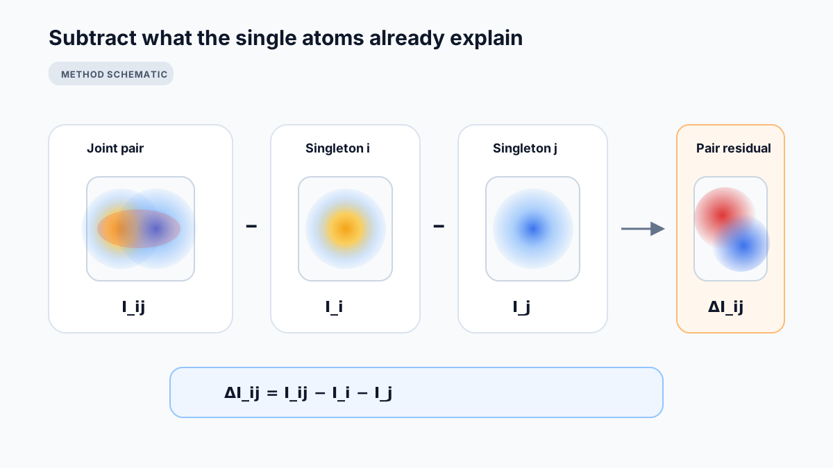
Calculate atoms i and j together, then subtract both matched singleton images. What remains is the pair-specific image contribution. A zero field would mean exact one-body additivity for that pair under the tested configuration.
Irreducible pair contribution
The pair contribution is image content present in the joint pair calculation that cannot be represented by the two matched singleton responses.
Subtract what the single atoms already explain
What if every pair is still not enough?
For three atoms, first construct the one-body sum and then add all three exact matched pair contributions. Compare that pair-corrected reconstruction with the full three-atom calculation. Any field that remains cannot be represented by the matched one- and two-body terms used in that reconstruction.
Irreducible three-body image term
This is an image-level inclusion–exclusion residual. It is not a direct count of microscopic three-particle scattering paths.
Build the image in layers
Technical depth: General subset form
The same bookkeeping can be written recursively for any matched atomic subset T. The tutorial only needs the one-, two-, and three-atom cases above.
Now test the idea against the frozen study
The preceding figures were explanatory. From this point onward, the tutorial switches to Paper 1 evidence. The numerical plots below use frozen result records or retained publication figures, and their captions state the evidence boundary explicitly. Numerical values and qualifications were rechecked against the final frozen Paper 1 evidence state on 2026-09-24.
Pair non-additivity is strongly geometry dependent
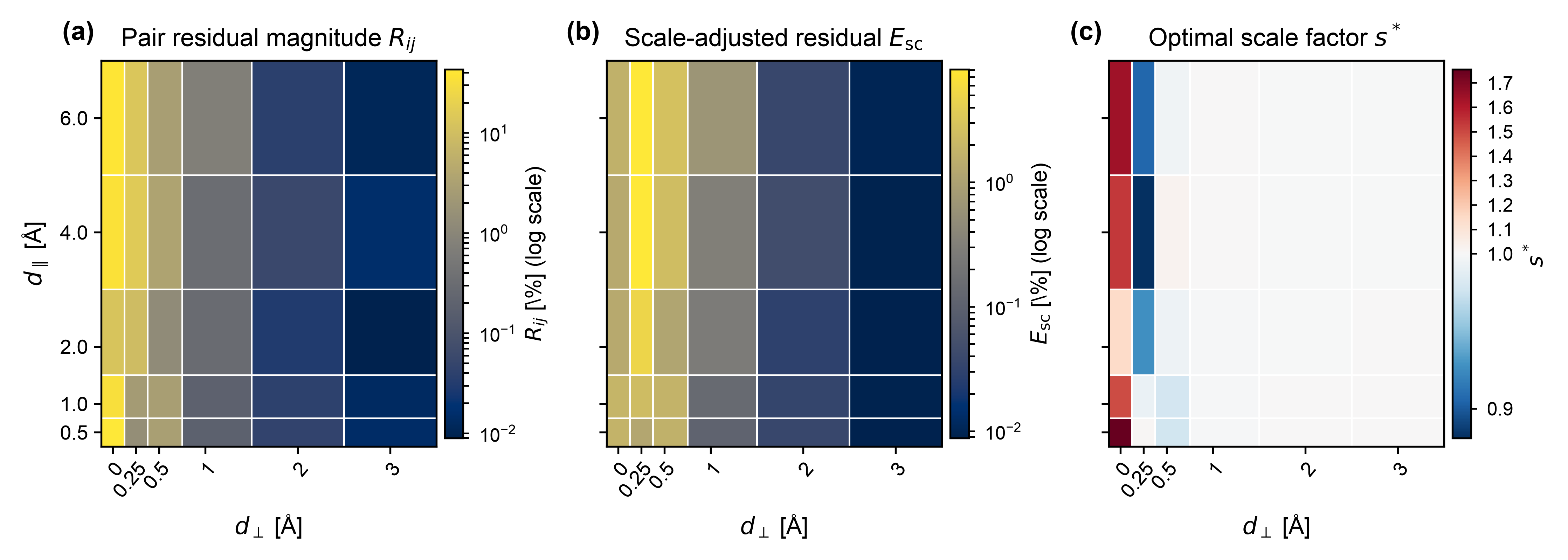
Read one cross-section before reading the whole map
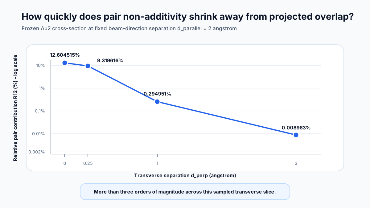
At fixed beam-direction separation d_parallel = 2 Å, the 0.50 Å production-map relative pair contribution R_12 = ||ΔI_12||_2 / ||I_12||_2 changes from 12.604515% at exact projected overlap to 9.319616% at d_perp = 0.25 Å, 0.294951% at 1 Å, and 0.008963% at 3 Å.
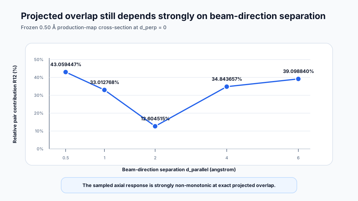
The complementary exact-overlap cross-section holds d_perp = 0 and varies d_parallel: 43.059447%, 33.012768%, 12.604515%, 34.843657%, and 39.098840% at 0.5, 1, 2, 4, and 6 Å. Together the two slices show both orders-of-magnitude transverse suppression and strongly non-monotonic axial dependence. The result should not be simplified to a universal one-distance decay law.
The same result as one simple cross-section
Projected overlap still depends strongly on beam-direction separation
A sophisticated correction can pass and still be unnecessary
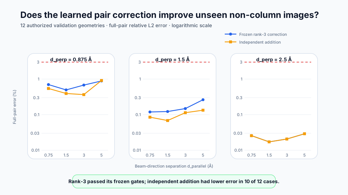
Passing a gate is not the same as earning extra complexity
Here rank 3 means that, after translating pair-residual images to a common projected midpoint, the compact representation retained three singular-value-decomposition (SVD) spatial modes. The rank, applicability boundary, and interpolation rule were fixed using development data before independent validation.
Across the 12 authorized non-column validation geometries, the frozen rank-3 model had median full-image error 0.1353% and maximum 0.8862%. Pure matched singleton addition had median 0.0992% and maximum 0.9127%, and was more accurate in 10 of the 12 cases.
The scientifically useful conclusion is not that the pair residual is unreal. It is that these complete non-column pair images were already approximately additive at the sub-percent level, so the learned correction was not supported as an overall predictive improvement in this tested regime.
Full-image accuracy and residual accuracy are different questions
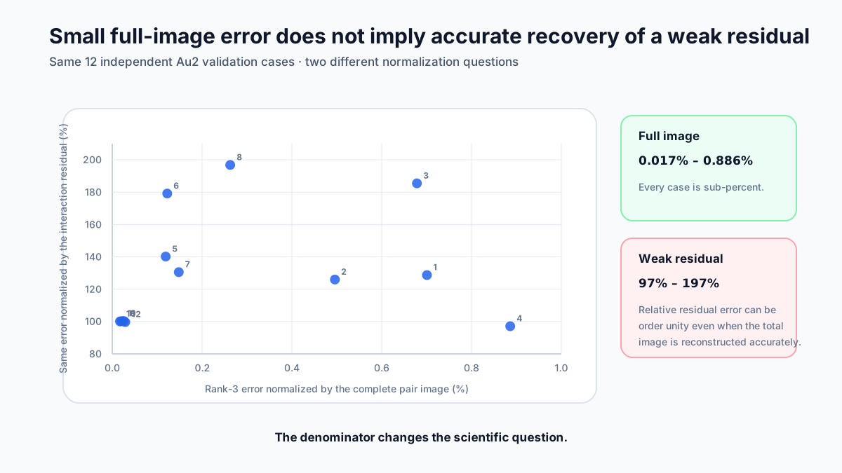
Technical depth: Why relative L2 here?
The primary Paper 1 metric is not a human-perceptual similarity score. Compared images share the same physical scan grid, atomic coordinates, microscope configuration, and intensity convention, so each pixel represents the same physical probe position and an intensity mismatch is part of the reconstruction error.
Relative L2 measures the complete registered image-field discrepancy relative to the reference image. Residual normalization changes the scientific target from full-image fidelity to fidelity of the weaker non-additive component. Global scale adjustment diagnoses amplitude versus spatial mismatch, while cosine similarity checks whether residual shape persists under refinement.
SSIM and human visual judgments address perceptual similarity instead. That is a separate observer question, not the acceptance target here.
Why the denominator changes the conclusion
When ΔI_12 is tiny compared with I_12, an error that is negligible relative to the full image can be comparable to the entire residual itself. The validation therefore supports approximate additivity of the full image. It does not establish that the weak pair residual was reconstructed accurately relative to its own norm.
Under strong overlap, every exact pair can still be insufficient
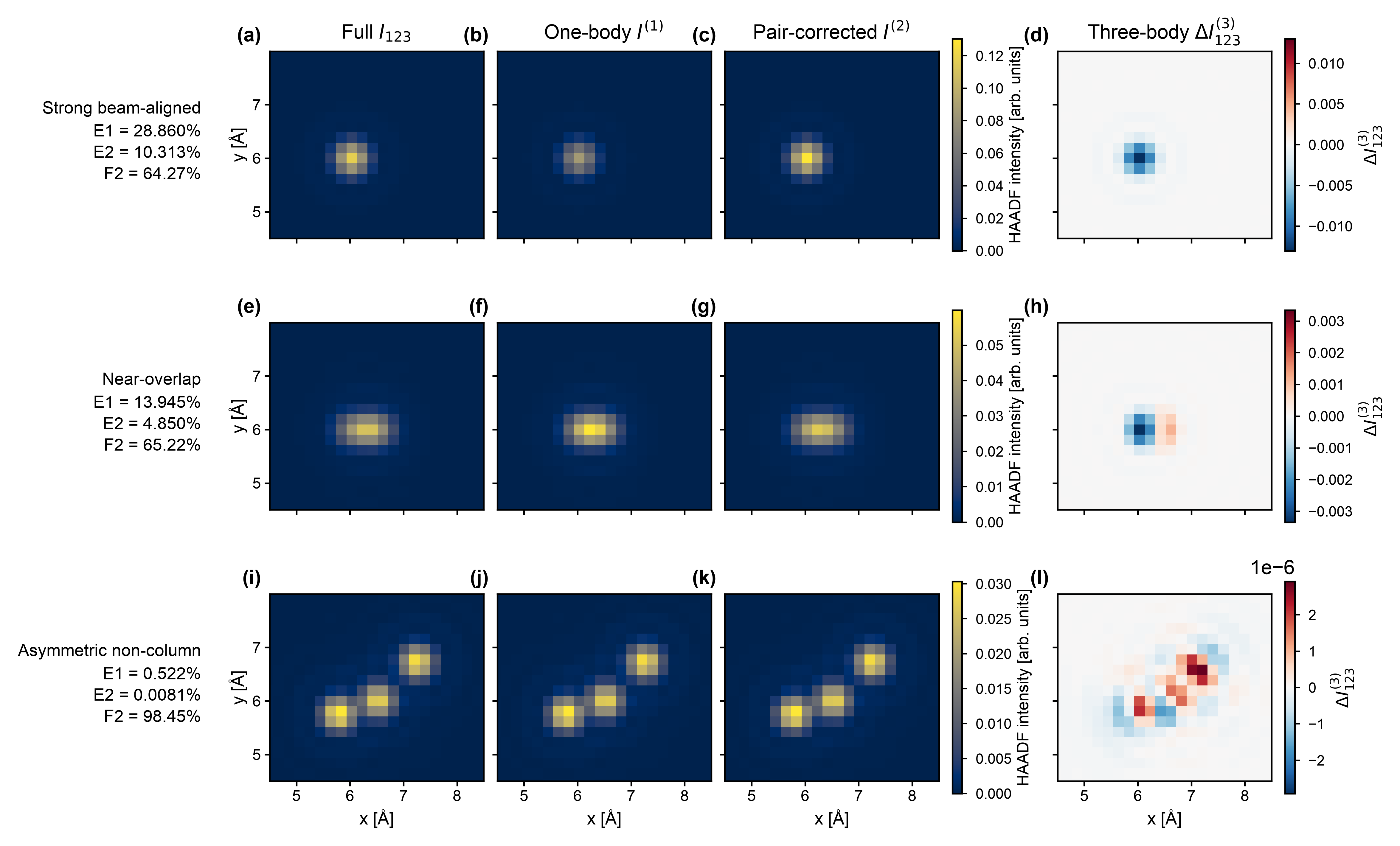
The same decomposition gives three very different answers
Beam aligned: E1 = 28.860416%, E2 = 10.313025%, F2 = 64.265848%. Near overlap: E1 = 13.944548%, E2 = 4.849940%, F2 = 65.219811%. Asymmetric non-column: E1 = 0.522053%, E2 = 0.008114%, F2 = 98.445841%.
E1 is the singleton-only full-image error. E2 is the error after every exact matched pair term is included, and is also the full-image-normalized magnitude of the remaining three-atom residual. F2 asks what fraction of the original singleton discrepancy the pairs removed. Improvement and final adequacy are therefore separate questions.
The strong-overlap residuals survive the tested refinement
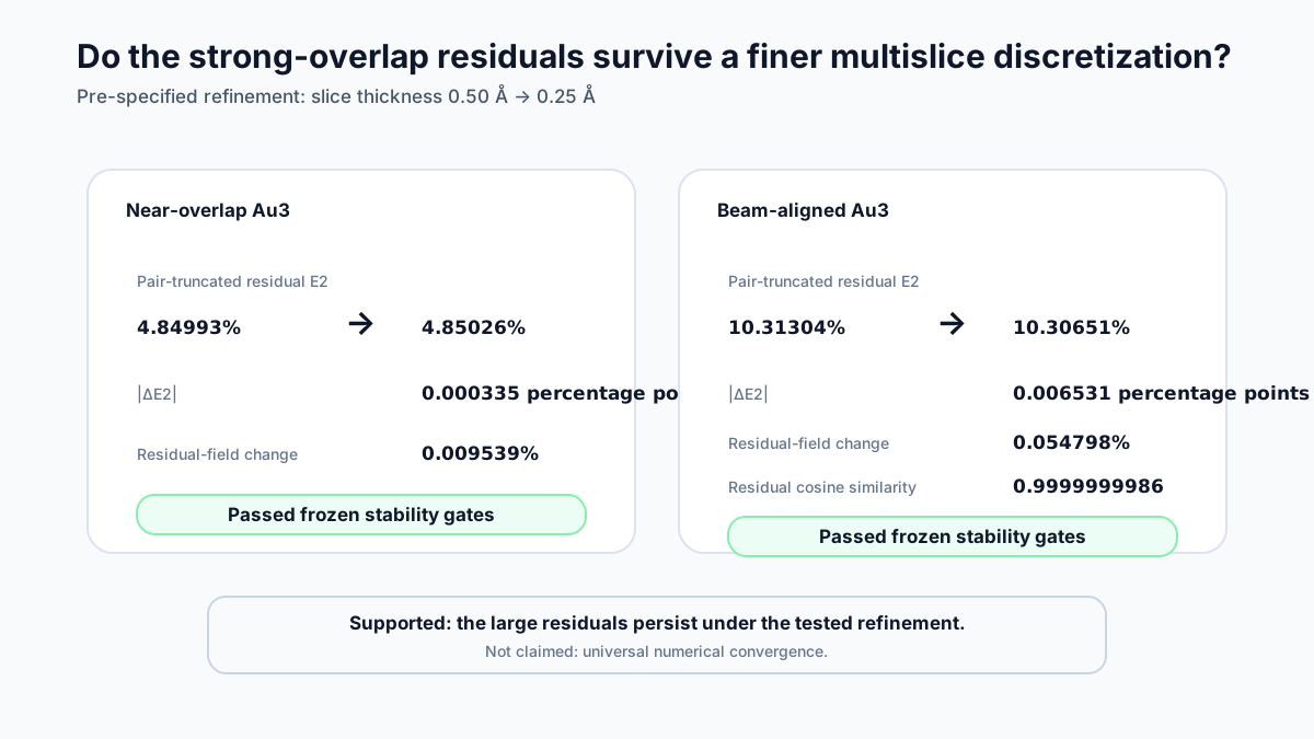
A skeptical alternative was tested directly
For near overlap, reducing slice thickness from 0.50 to 0.25 Å changed E2 by only 0.000335 percentage points and the residual field by 0.009539% relative to the refined residual norm. For beam alignment, E2 changed by 0.006531 percentage points; the residual field changed by 0.054798% and had cosine similarity 0.9999999986.
After the original confirmatory protocol, the asymmetric non-column control was also subjected to a separately frozen reviewer-motivated 0.50-to-0.25 Å slice-thickness check. Its E1, E2, and F2 changes were 0.0001305, 0.00000145, and 0.000665 percentage points; the residual field changed by 0.202% with cosine similarity 0.999998. It passed the reused stability tolerances, but remains post-hoc robustness evidence.
A second post-review check expanded the beam-aligned lateral cell from 15×12 to 21×18 Å while preserving relative geometry and scan registration. E2 changed from 10.3130% to 10.2920%; the irreducible residual field changed by 0.783% and retained cosine similarity 0.99999947. This supports persistence under the tested padding, not universal cell-size convergence.
The 0.75 Å value came from a stopped, ordered search
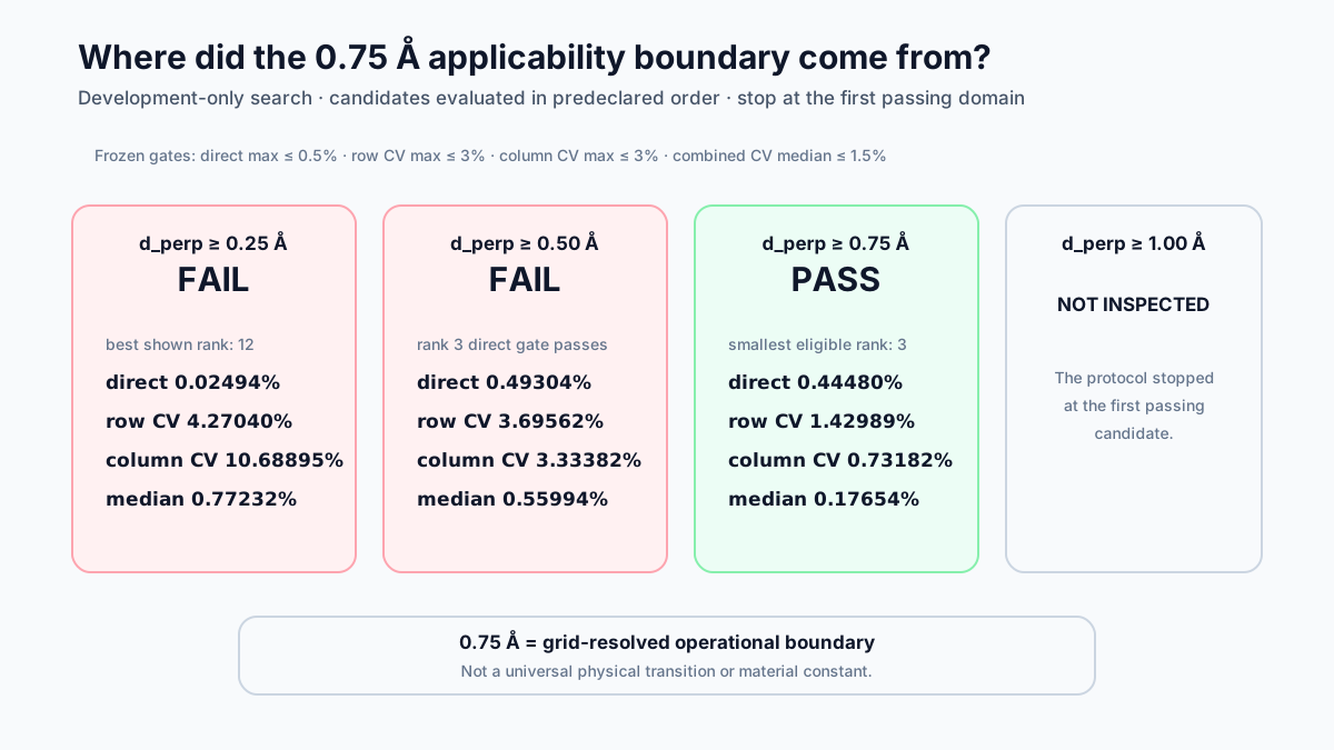
What the boundary does—and does not—mean
The candidate domains were d_perp ≥ 0.25, 0.50, 0.75, and 1.00 Å, evaluated in that fixed order. The 0.25 and 0.50 Å domains failed cross-validation criteria even when direct reconstruction was accurate. The 0.75 Å domain was the first to pass every frozen gate, with rank 3 the smallest eligible representation, so the protocol stopped before inspecting 1.00 Å.
This is not a universal physical transition at 0.75 Å. It identifies the first tested development domain in which the unchanged compact representation generalized adequately according to study-specific decision criteria.
The scientific lesson
For the configurations tested here, effective image order is geometry dependent. Independently tested non-column Au2 images were already approximately additive at the sub-percent full-image level. Under strong projected overlap, pair non-additivity became much larger; in the tested beam-aligned and near-overlap Au3 controls, even every exact pair contribution left substantial higher-order image residuals. Use the simplest image representation that the geometry and evidence support.
Scope and limitations
The study uses controlled static-lattice multislice calculations for Au2 and Au3 under fixed imaging conditions. Frozen-phonon thermal diffuse scattering was not included, nor were post-simulation shot noise or detector-degradation models. Scan-spacing convergence was not established, and lateral-cell sensitivity was tested only in the later beam-aligned robustness check rather than as a systematic convergence study. The reported magnitudes and 0.75 Å development boundary therefore characterize this deterministic simulation study, not finite-temperature experimental detectability thresholds or universal material laws.
Concept glossary
| Term | Meaning in this tutorial |
|---|---|
| Matched subset | Selected atoms keep their exact coordinates from the full structure while the other atoms are removed and the comparison configuration is kept fixed. |
| One-body reconstruction | The sum of all matched singleton images. |
| Pair residual ΔI_ij | The part of a matched two-atom image not explained by adding its two matched singleton images. |
| Rank-3 representation | A compact development-stage description of aligned pair-residual images using three retained SVD spatial modes; the rank was fixed before independent validation. |
| Higher-order residual | What remains after the included lower-order matched contributions are subtracted; an image-level inclusion–exclusion quantity, not a unique microscopic scattering path. |
| R_12 | Pair-residual magnitude normalized by the complete two-atom image. |
| E1 | Full-image error of the singleton-only reconstruction. |
| E2 | Full-image error after every exact matched pair term is included for the Au3 controls. |
| F2 | Fraction of the original one-body discrepancy removed by the exact pair terms. |
| Operational boundary | A boundary selected by a declared numerical rule over the sampled development grid, not automatically a physical transition. |
| Multislice simulation | A numerical electron-microscopy method that propagates the electron wave through successive slices of the specimen potential. |
| Static lattice | A calculation with atoms fixed at specified positions; no frozen-phonon thermal-displacement ensemble is included here. |
| Preregistered / frozen gate | An acceptance criterion fixed before the confirmatory validation result is inspected, so the threshold is not adjusted to fit that result. |
| Post-hoc comparison | An analysis performed after the confirmatory decision was fixed; informative, but not presented as a preregistered superiority test. |
| Relative L2 error | Magnitude of the registered pixelwise error field divided by the reference-image magnitude; used here for physical reconstruction fidelity rather than human-perceptual similarity. |
| Scale-adjusted residual | Error remaining after fitting one global multiplicative intensity scale; used diagnostically to separate overall amplitude mismatch from spatial-field mismatch. |
| Cosine similarity | Field-shape alignment of two residual vectors independent of overall magnitude; used here in numerical-robustness checks. |
Check your understanding
1. Why is a bright HAADF-STEM feature not a direct picture of an atom?
2. If ΔI_12 = 0, what does that say about the matched two-atom image?
3. Why can geometries with similar three-dimensional atom–atom distance behave differently when d_perp and d_parallel differ?
4. The frozen rank-3 Au2 representation passed its preregistered gates, yet simple addition had lower error in 10 of 12 post-hoc comparisons. What is the defensible conclusion?
5. What does a substantial Au3 E2 show, and what does it not identify?
6. Why should the 0.75 Å value not be interpreted as a universal experimental threshold?
Answers: Check your understanding
1. The feature is an imaging-system response, not the physical outline of the atom.
2. The joint pair image is exactly reproduced by the two matched singleton images at image level for that tested configuration.
3. Projected overlap and propagation along the beam are different geometric controls; the frozen evidence shows strong transverse suppression and non-monotonic axial dependence.
4. The tested non-column full images are already approximately additive at sub-percent error, so the learned correction is not scientifically necessary there despite being a real fitted correction.
5. Substantial E2 means exact pair terms do not fully reconstruct the complete image; it does not identify a unique microscopic three-particle scattering pathway or many-body potential.
6. The value is the first sampled development boundary that passed the frozen numerical criteria, so it is operational and grid-resolved rather than a universal physical transition.
Sources and further reading
Geometry-Resolved Few-Body Decomposition of HAADF-STEM Image Formation. Submission-ready unpublished manuscript. The first nine explanatory schematics teach the method. Within the later evidence section, two figures reuse retained frozen publication figures from the research repository; the remaining evidence figures visualize frozen production-map cross-sections, validation, normalization, refinement, and boundary-selection records. The underlying research arrays remain governed by the durable Paper 1 archive rather than being duplicated into the portfolio.